ondisk
Disk-backed Analysis
Emerging spatial omics instruments are capable of generating millions of cells and transcripts as well as large high-resolution images. Existing software packages mostly use default in-memory storage (provided by built-in R objects) for both feature vs observations matrices and biological images of spatial omics datasets, however this approach both slow and inefficient. A common alternative is to use novel disk-backed data objects in R that allow data to sit in the disk, while efficiently stream data to memory for processing and analysis.
We use BPCells and ImageArray packages to store large feature matrices and images to accelerate operations. Here BPCells allows users access and operate on large feature matrices or clustering/spatial analysis, while ImageArray provides image pyramids to allow fast access to large microscopy images.
You can download these packages using our bundle package VoltRonStore from GitHub using devtools. Installing VoltRonStore will install all dependencies of VoltRon that facilitates on-disk support.
devtools::install_github("BIMSBbioinfo/VoltRonStore")
library(BPCells)
library(ImageArray)
Spot-level Analysis (VisiumHD)
We first have to download some packages that are necessary to import
datasets from .parquet and .h5 files provided
by the VisiumHD readouts.
if(!requireNamespace("arrow"))
  install.packages("arrow")
if(!requireNamespace("rhdf5"))
  BiocManager::install("rhdf5")
We use the importVisiumHD function to start analyzing the data. The data has 393401 spots which we will use disk-backed methods to efficiently manipulate, analyze and visualize these spots.
The VisiumHD readouts provide multiple bin sizes which are aggregated versions of the original 2\(\mu\)m \(x\) 2\(\mu\)m capture spots. The default bin sizes are (i) 2\(\mu\)m \(x\) 2\(\mu\)m, (ii) 8\(\mu\)m \(x\) 8\(\mu\)m and (iii) 16\(\mu\)m \(x\) 16\(\mu\)m.
hddata <- importVisiumHD(dir.path = "VisiumHD/outs/",
                         bin.size = "8",
                         resolution_level = "hires")
On-Disk VoltRon Objects
We can now save the VoltRon object to disk, large matrices and images
will be written to either hdf5 or zarr
files depending on the format argument, and the rest of
the R object would be written to an .rds file, both under
the designated output.
hddata <- saveVoltRon(hddata, format = "HDF5VoltRon", output = "data/VisiumHD")If you want you can load the VoltRon object from the same path as you have saved.
hddata <- loadVoltRon("data/VisiumHD/")Analysis and Visualization
The BPCells package provides fast methods to achieve operations common to single cell analysis such as filtering, normalization and dimensionality reduction. Here we have an example of single-cell like clustering of VisiumHD bins which is efficiently clustered.
spatialpoints <- vrSpatialPoints(hddata)[as.vector(Metadata(hddata)$Count > 10)]
hddata <- subset(hddata, spatialpoints = spatialpoints)
hddata <- normalizeData(hddata, sizefactor = 10000)
hddata <- getFeatures(hddata, n = 3000)
selected_features <- getVariableFeatures(hddata)
hddata <- getPCA(hddata, features = selected_features, dims = 30)
hddata <- getUMAP(hddata, dims = 1:30)
We can now visualize genes over embedding or spatial plots.
vrEmbeddingFeaturePlot(hddata, features = "Nrgn", embedding = "umap")
vrSpatialFeaturePlot(hddata, features = "Nrgn")
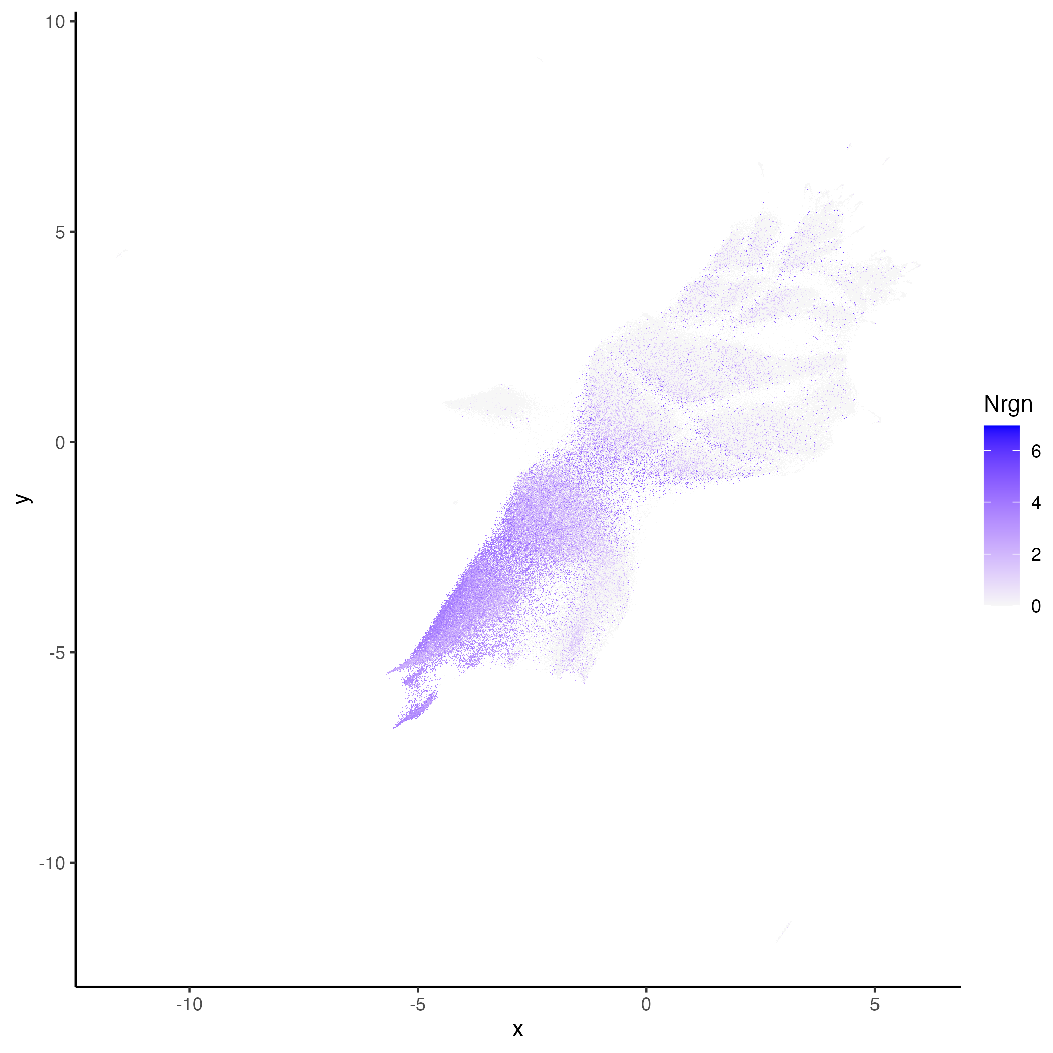
|
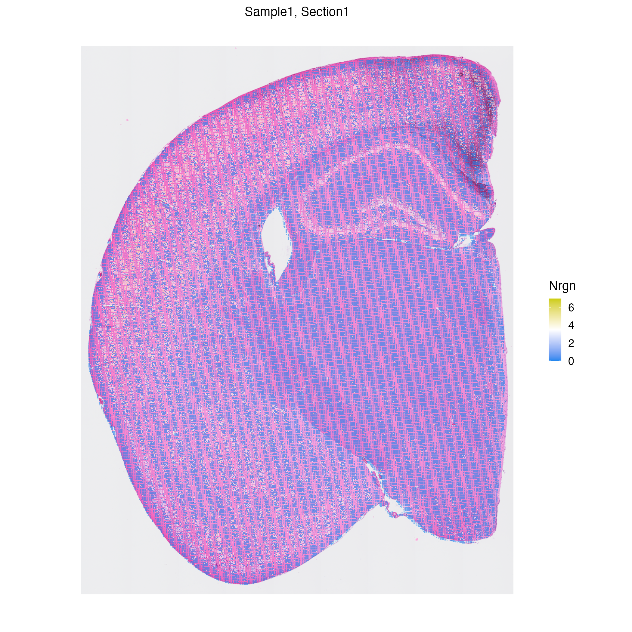
|
Cell-level Analysis (Xenium)
To demonstrate that VoltRon facilitates large data analysis on single cell level, we use an atlas level dataset generated by the Xenium in situ platform, specifically a spatially captured one day old mouse pup data generated using the Mouse Tissue Atlassing panel (379 genes). The mouse data includes around 1.3 million cells which we store on disk to efficiently manipulate, analyze and visualize.
See Whole Mouse Pup Preview to learn more than the panel and the readout.
# dependencies
if(!requireNamespace("RBioFormats"))
  BiocManager::install("RBioFormats")
if(!requireNamespace("arrow"))
  install.packages("arrow")
if(!requireNamespace("rhdf5"))
  BiocManager::install("rhdf5")

# import Xenium data
Xen_R1 <- importXenium("Xenium_pup/outs/",
                       sample_name = "XeniumR1",
                       resolution_level = 3,
                       overwrite_resolution = TRUE)
On-Disk VoltRon Objects
We can now save the VoltRon object to disk, large matrices and images
will be written to either hdf5 or zarr
files depending on the format argument, and the rest of
the R object would be written to an .rds file, both under
the designated output.
Xen_R1 <- saveVoltRon(Xen_R1, format = "HDF5VoltRon",
                      output = "data/Xenium_pups", replace = TRUE)
If you want you can load the VoltRon object from the same path as you have saved.
Xen_R1 <- loadVoltRon("data/Xenium_pups/")Analysis and Visualization
The BPCells package provides fast methods to achieve operations common to single cell analysis such as filtering, normalization and dimensionality reduction. Here we have an example of single-cell like clustering of VisiumHD bins which is efficiently clustered.
spatialpoints <- vrSpatialPoints(Xen_R1)[as.vector(Metadata(Xen_R1)$Count > 10)]
Xen_R1 <- subset(Xen_R1, spatialpoints = spatialpoints)
Xen_R1 <- normalizeData(Xen_R1, sizefactor = 10000)
We now visualize the localization of three markers, specifically Dsc3, Clec4f, Gfap; that point to the skin, liver and brain of the pup, respectively. The n.tile parameter controls the level of rasterization of gene expression or metadata columns to speed up data visualization. Here, n.tile=400 bins expression and metadata measures into 400 chunks along the x-and y-axis of the image.
vrSpatialFeaturePlot(Xen_R1, features = c("Dsc3", "Clec4f", "Gfap"), n.tile = 400, alpha = 1, ncol = 3, log = TRUE)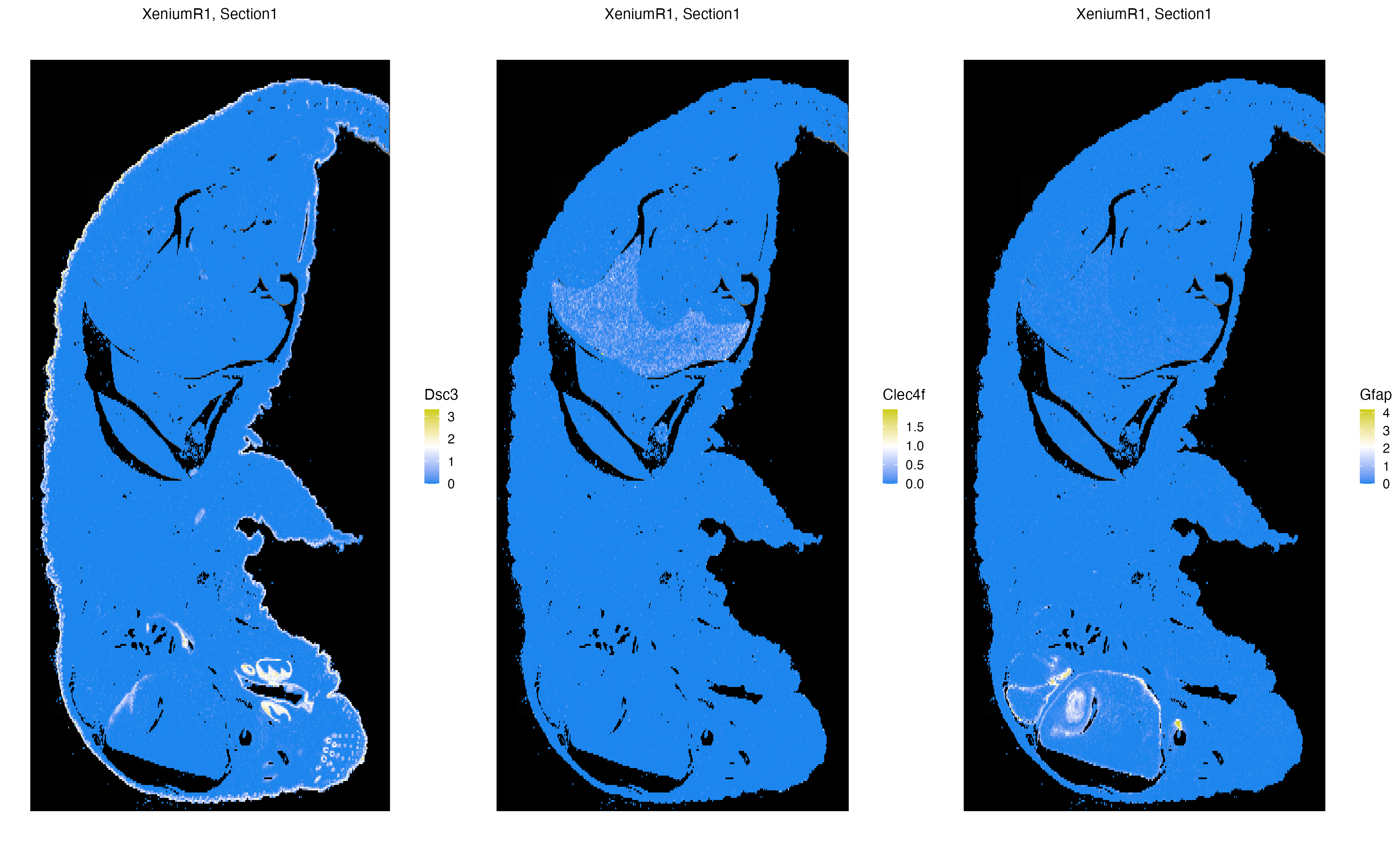
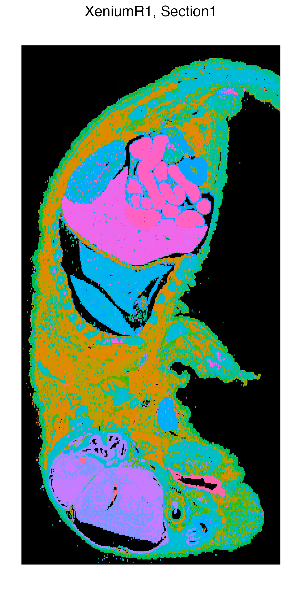
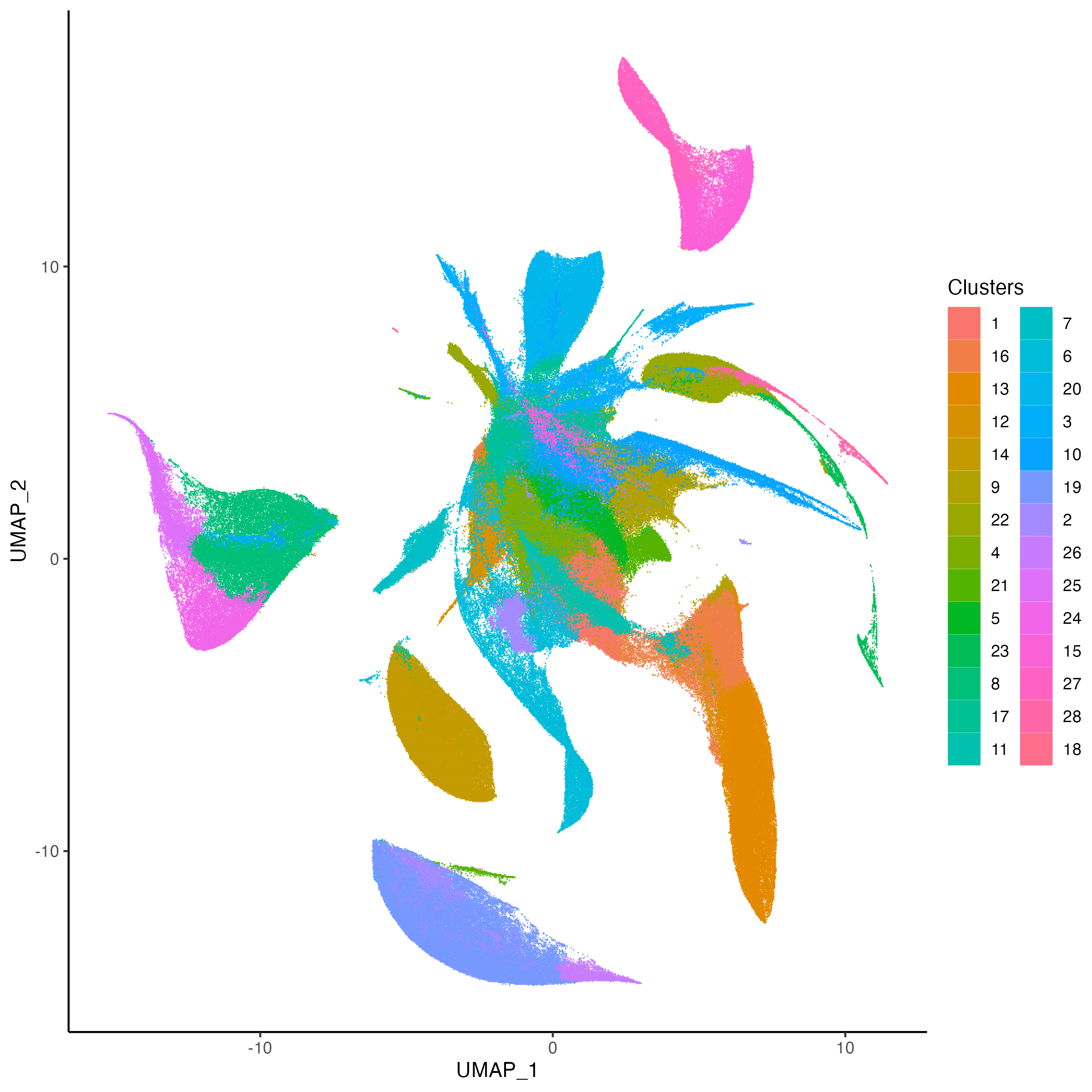
We now learn PCA and UMAP embeddings of the mouse data, and cluster using shared nearest neighbor (SNN) graph.
Xen_R1 <- getPCA(Xen_R1, dims = 30)
Xen_R1 <- getUMAP(Xen_R1, dims = 1:30)
Xen_R1 <- getProfileNeighbors(Xen_R1, dims = 1:30, k = 10, method = "SNN")
Xen_R1 <- getClusters(Xen_R1, resolution = 0.7, label = "Clusters", graph = "SNN")

library(patchwork)
g1 <- vrSpatialPlot(Xen_R1, group.by = "Clusters", n.tile = 400,
                    alpha = 1, legend.loc = "none")
g2 <- vrEmbeddingPlot(Xen_R1, group.by = "Clusters", embedding = "umap")
g1 | g2
|
|
Spatial Data Alignment
The image registration workflow in the Spatial Data Alignment tutorial can also be conducted using disk-backed methods of the VoltRon package.
# dependencies
if(!requireNamespace("RBioFormats"))
  BiocManager::install("RBioFormats")
if(!requireNamespace("arrow"))
  install.packages("arrow")
if(!requireNamespace("rhdf5"))
  BiocManager::install("rhdf5")
library(VoltRon)

# import Xenium data
Xen_R1 <- importXenium("Xenium_R1/outs", sample_name = "XeniumR1", resolution_level = 3)

# import H&E image
Xen_R1_image <- importImageData("Xenium_FFPE_Human_Breast_Cancer_Rep1_he_image.tif",
                                sample_name = "XeniumR1image",
                                image_name = "H&E")
We can save both Xenium and H&E (image) datasets to disk before using the mini Shiny app for registration
Xen_R1_disk <- saveVoltRon(Xen_R1,
                           format = "HDF5VoltRon",
                           output = "data/Xen_R1_h5", replace = TRUE)
Xen_R1_image_disk <- saveVoltRon(Xen_R1_image,
                                 format = "HDF5VoltRon",
                                 output = "data/Xen_R1_image_h5", replace = TRUE)
These disk-based datasets can then be loaded from the disk easily.
Xen_R1_disk <- loadVoltRon("../data/OnDisk/Xen_R1_h5/")
Xen_R1_image_disk <- loadVoltRon("../data/OnDisk/Xen_R1_image_h5/")
VoltRon stores large images as pyramids to increase interactive
visualization efficiency. This storage strategy allows shiny apps to
zoom in to tissue niches in a speedy fashion. VoltRon incorporates
Image_Array objects (https://github.com/BIMSBbioinfo/ImageArray) to define
these pyramids.
vrImages(Xen_R1_image_disk, as.raster = TRUE)Image_Array Object
Series 1 of size (3,27587,20511)
Series 2 of size (3,13794,10256)
Series 3 of size (3,6897,5128)
Series 4 of size (3,3449,2564)
Series 5 of size (3,1725,1282)
Series 6 of size (3,863,641)
Series 7 of size (3,432,321) We can now visualize and align the Xenium and H&E objects.
# Align spatial data
xen_reg <- registerSpatialData(object_list = list(Xen_R1_disk, Xen_R1_image_disk))# transfer aligned H&E to Xenium data
Xenium_reg <- xen_reg$registered_spat[[2]]
vrImages(Xen_R1_disk[["Assay1"]], name = "main", channel = "H&E") <- vrImages(Xenium_reg, name = "H&E_reg")
# visualize
vrImages(Xen_R1_disk, channel = "H&E", scale.perc = 10)