Importing Spatial Data
Analysis of Images
VoltRon is a spatial omics analysis platform that allows storing a large amount of spatially resolved datasets. As opposed to datasets with either supracellular (spot-level) or cellular resolutions, one might analyze image datasets and pixels to characterize the morphology of a tissue section.
Here, images can also be used to build VoltRon objects where pixels (or tiles) are defined as spatial points, and then can also be used for multiple downstream analysis purposes.
Importing Images (H&E)
In this use case, we will analyze the H&E image derived from a tissue section that was first analyzed by The 10x Genomics Xenium In Situ platform. Three tissue sections were cut from a single formalin-fixed, paraffin-embedded (FFPE) breast cancer tissue block. A 5 \(\mu\)m section was used to generate a single Xenium replicate. The H&E staining was performed on the tissue after the Xenium run.
More information on the Xenium and the study can be also be found on the BioRxiv preprint. You can download the H&E image from the 10x Genomics website as well (specifically, import the Post-Xenium H&E image (TIFF) data).
We incorporate importImageData to convert an image into a tile/pixel-based spatial dataset.
Xen_R1_image <- importImageData("Xenium_FFPE_Human_Breast_Cancer_Rep1_he_image.tif",
                                sample_name = "XeniumR1image",
                                image_name = "H&E", tile.size = 100)
Xen_R1_image
VoltRon Object
XeniumR1image:
Layers: Section1
Assays: ImageData(Main)
Features: main(Main) vrImages(Xen_R1_image, scale.perc = 2)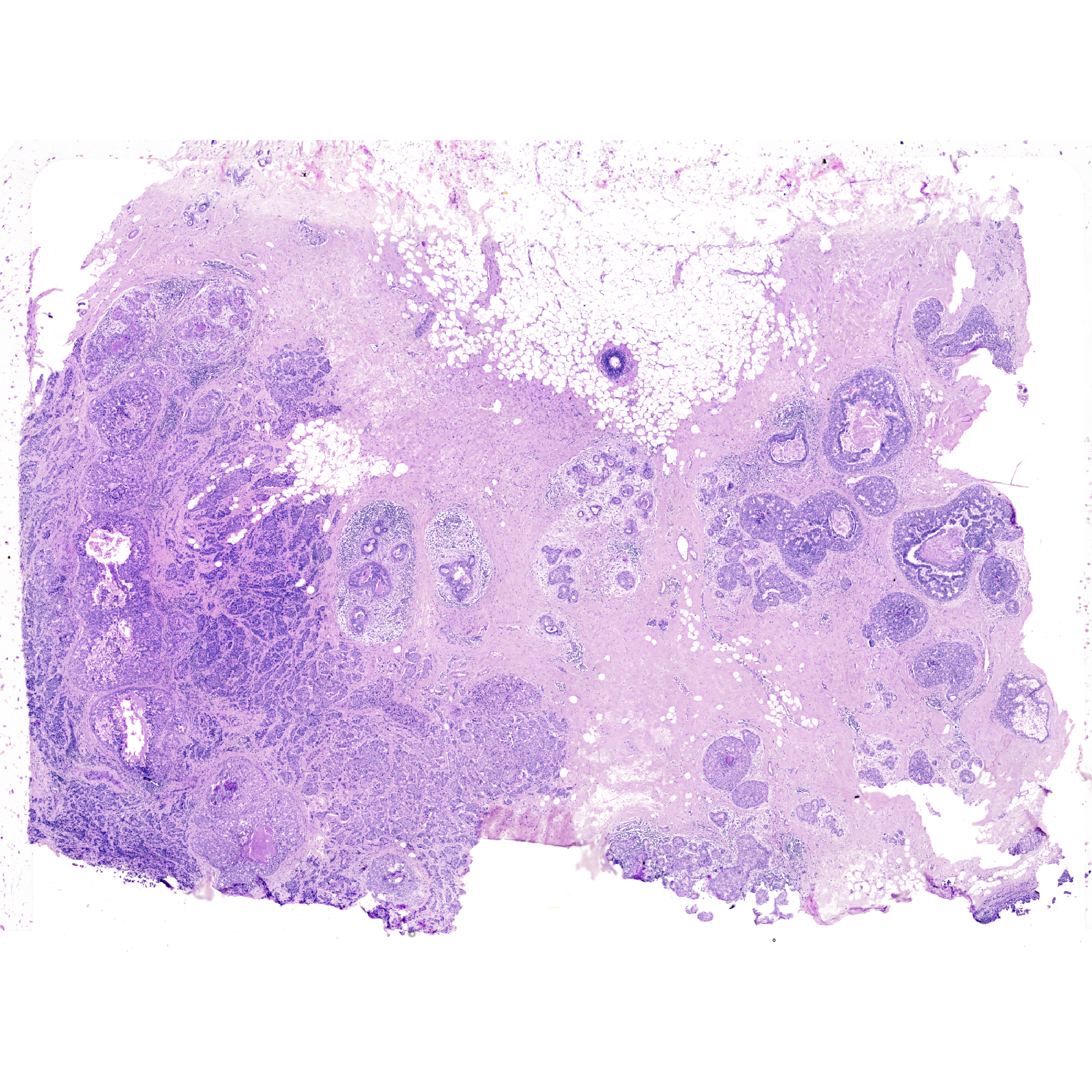
Building Datasets for Tiles
The VoltRon object stores the metadata information and localization of all tiles in the image. These tiles, like any observation, can be analyzed independently where you can reduce its dimensionality to perform clustering later.
head(Metadata(Xen_R1_image)) id assay_id Assay Layer Sample
<char> <char> <char> <char> <char>
1: tile1_2c05fc Assay1 ImageData Section1 XeniumR1image
2: tile2_2c05fc Assay1 ImageData Section1 XeniumR1image
3: tile3_2c05fc Assay1 ImageData Section1 XeniumR1image
4: tile4_2c05fc Assay1 ImageData Section1 XeniumR1image
5: tile5_2c05fc Assay1 ImageData Section1 XeniumR1image
6: tile6_2c05fc Assay1 ImageData Section1 XeniumR1imageEach row is associated with a tile of parsed from the image, and the users can define additional metadata columns afterwards.
nrow(Metadata(Xen_R1_image))[1] 24888In order to generate data values from image tiles, we can treat each pixel of a tile as a data dimension (in this case, by 200x200 tiles we have 40000 pixels, thus dimensions). We generate this dataset as below:
Xen_R1_image <- generateTileData(Xen_R1_image)
dim(vrData(Xen_R1_image))
[1] 40000 13974Dimensionality Reduction
We can now reduce the dimensionality of these pixel intensities using PCA and visualize the data variability across tiles. The data matrix we generated with the generateTileData earlier will be used here similar to gene/protein expression datasets, where we reduce 40000 variables (each associated with a pixel) to a manageable number, say 15.
Xen_R1_image <- getPCA(Xen_R1_image, dims = 15)
Xen_R1_image <- getUMAP(Xen_R1_image)
vrEmbeddingPlot(Xen_R1_image, embedding = "umap", group.by = "Sample")![]()
Clustering
Here, the dimensionally reduced image tiles can be clustered using either graph clustering approaches or kmeans clustering depending on the choice.
Xen_R1_image <- getProfileNeighbors(Xen_R1_image, data.type = "pca",
                                    k = 10, method = "SNN", dims = 1:15)
Xen_R1_image <- getClusters(Xen_R1_image, resolution = 1.0,
                            label = "Cluster_snn", graph = "SNN")
Here, we visualize the transparent clustering information of tiles by rasterizing the tiles into larger sizes to increase plotting speed where we can see the distinction between different tissue niches of the image.
g1 <- vrSpatialPlot(Xen_R1_image, group.by = "Cluster_snn",
                    alpha = 0.5, n.tile = 100)
g2 <- vrEmbeddingPlot(Xen_R1_image, embedding = "umap",
                      group.by = "Cluster_snn")
g1 | g2 |
|
|
Image Foundation Models
Using VoltRon we can also integrate tile-level spatial entities and image tiles with existing image foundation models such as DinoV2 or UNI.
We can parse tiles from VoltRon, and get embedding values from a Foundation model to conduct downstream clustering using PCA and kmeans clustering.
Importing Images (H&E)
We first import the H&E image to VoltRon. This time we will set the tile size to 128 which will generate 34400 tiles on the breast cancer tissue.
Xen_R1_image <- importImageData("Xenium_FFPE_Human_Breast_Cancer_Rep1_he_image.tif",
                                sample_name = "XeniumR1image",
                                image_name = "H&E", tile.size = 128)
Xen_R1_image@metadata
VoltRon Metadata Object
This object includes:
34400 tiles Add External Embeddings
We will now load and add the DinoV2 embeddings as additional
embedding data before analysis and clustering. Here, we use
overwrite argument (default is FALSE) as a
safe-guard for overwriting already existing embeddings with the same
name, i.e. type = "dinov2", but if the an embedding with
name dinov2 doesn’t exist, this will be overlooked. You can
download the DinoV2 embeddings from here.
# get embed data
dinov2_embed <- readRDS("img_128_processed.rds")
ind <- sapply(vrSpatialPoints(Xen_R1_image), function(x) strsplit(x, split = "_")[[1]][1])
dinov2_embed <- dinov2_embed[ind,]
rownames(dinov2_embed) <- vrSpatialPoints(Xen_R1_image)

# import DinoV2 embedding
vrEmbeddings(Xen_R1_image, type = "dinov2", overwrite = TRUE) <-  dinov2_embed
Dimensionality Reduction
If we check the number of extracted features from the DinoV2 model, we see that its 1536 which we could further reduced using PCA and UMAP prior to clustering.
Xen_R1_image <- getPCA(Xen_R1_image, dims = 50, data.type = "dinov2")
Xen_R1_image <- getUMAP(Xen_R1_image)
vrEmbeddingPlot(Xen_R1_image, embedding = "umap", group.by = "Sample")![]()
Clustering
With the PCA embeddings generated from the DinoV2 embeddings now we can apply k-means clustering.
Xen_R1_image <- getClusters(Xen_R1_image, method = "kmeans",
                            label = "Cluster_kmeans", data.type = "pca",
                            nclus = 10)
vrEmbeddingPlot(Xen_R1_image, embedding = "umap", group.by = "Cluster_kmeans")
vrSpatialPlot(Xen_R1_image, group.by = "Cluster_kmeans", alpha = 1)|
|
|
We can zoom to certain locations over the tissue and visualize the tile-based embedding clusters over regions.
# interactive subsetting
Xen_R1_image_subset <- subset(Xen_R1_image, interactive = TRUE)
Xen_R1_image_subset <- Xen_R1_image_subset$subsets[[1]]

# visualization
vrSpatialPlot(Xen_R1_image_subset, group.by = "Cluster_kmeans", alpha = 0.5)![]()